
Arizona Water Observatory
Quick Start Blogs and Application Demonstrations
From Scattered Sources to a Single View: Getting Started with the Arizona Water Observatory
By Emily Wiggans & Sara Alonso Vicario, Center for Geospatial Solutions
If you work with water data in Arizona, you know the routine. You need to understand basin-scale conditions like how precipitation patterns in a given year relate to groundwater levels or active management area boundaries. So you open a browser, then another, and head to a few agency portals, each with its own format, interface, and quirks. By the time you’ve assembled the data you need, you’ve lost hours of research time.
The Arizona Water Observatory (AWO) was built to change that data discovery drudgery. It’s a web-based platform that brings together datasets that typically live across multiple institutions into a single, simple environment for exploration and analysis. Users can explore basin-scale conditions, combining surface water, groundwater, climate variables, and more. Whether you’re a researcher, planner, engineer, or water practitioner, the AWO is designed to help you spend less time finding and formatting data and more time exploring it.
This post walks you through the basics of the platform including:
- How to enter the platform
- How to add datasets
- How to customize your selected data and visualization
- How to compare and explore data.
If you’re new to the AWO and want to get a feel for how it could fit into your existing workflows, this is the place to start! If you’re already comfortable and ready to go deeper, skip to the end for additional resources.
Getting started
Head to https://arizonawaterobservatory.asu.edu/. A pop up screen welcomes you with a brief platform overview and links to the Glossary, FAQ, and User Guide tabs, which may be helpful resources in the future. When you’re ready, press “Continue” to open the interface. (You can always return to this information by clicking the “i” icon in the upper left of the top toolbar.
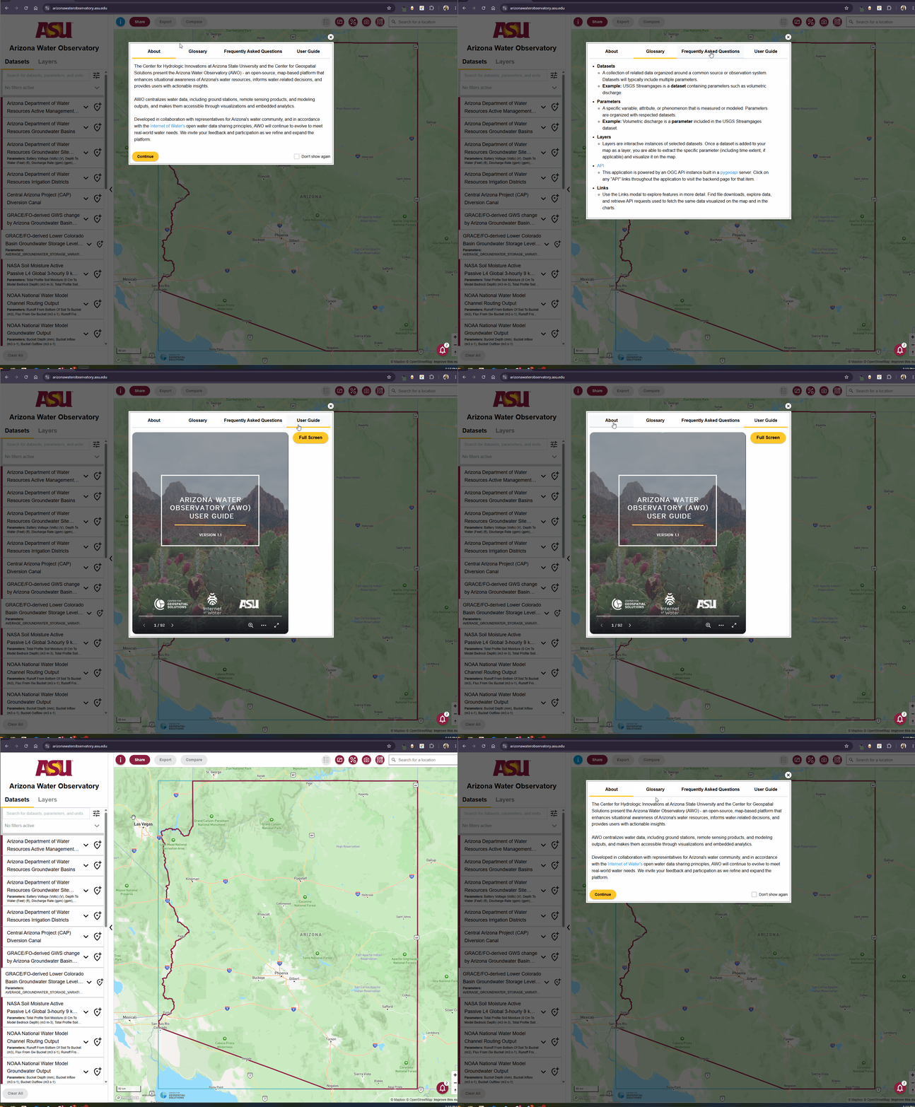
Navigate to arizonawaterobservatory.asu.edu. On the splash screen, note the Glossary, FAQ, and User Guide tabs, then click “Continue.” To return to this screen later, click the “i” icon in the upper left toolbar.
Adding your first datasets
There are a few ways to add data in the AWO. You can draw a specific area of interest or explore statewide data. For this walkthrough, we’ll add two datasets to the map: regulatory boundaries and precipitation data.
First, we’ll add Arizona’s Active Management Areas, or AMAs, which are regions established by the state’s1980 Groundwater Code where groundwater use is regulated to protect limited supply as populations grow. Then we’ll layer in PRISM precipitation data (short for Parameter-elevation Regressions on Independent Slopes Model), a dataset large enough that the platform will ask you to set a date range before loading. For this walkthrough, let’s explore the year 2023.
The result displays regulatory boundaries layered with monthly precipitation data, a task that would otherwise require pulling from two separate agency sources.
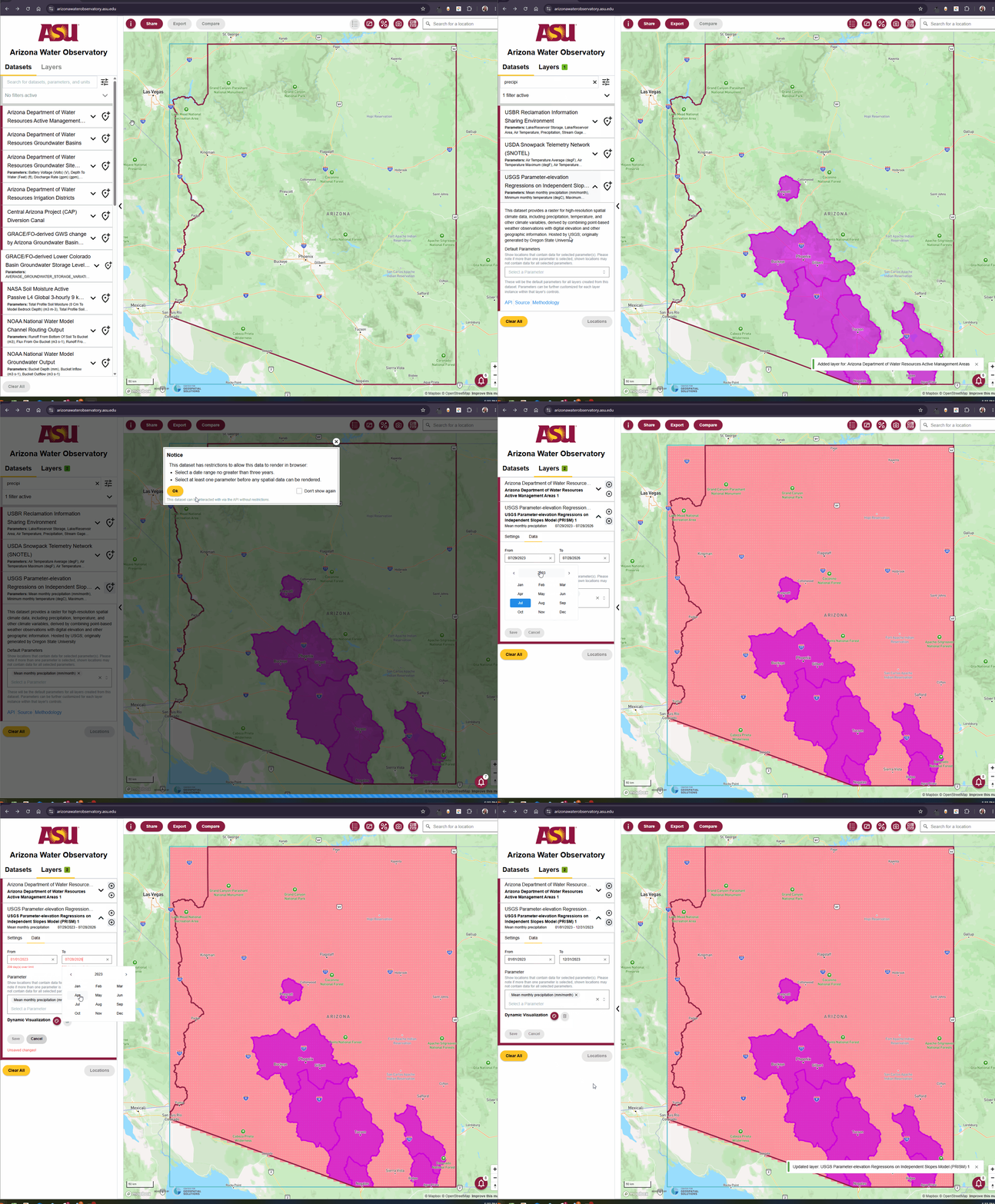
In the “Datasets” tab, find “Arizona Department of Water Resources Active Management Areas” and click the “pin+” icon to add it to the map. Then type “precipitation” into the search bar, locate the “USGS PRISM” dataset, select “Mean monthly precipitation (mm/month)” from the parameter dropdown, and click “pin+.” When prompted, set the date range to 01/01/2023 – 12/31/2023 and click “Ok.”
Customizing what you see
Once your datasets are loaded, the AWO gives you control over how they are displayed. For PRISM, you can rename the layer, adjust opacity, and choose a color ramp that makes precipitation patterns legible at a glance. In this example, we’ll use a Blue-Purple Palette with five groups, which will help intuitively distinguish wetter from drier areas across the state.
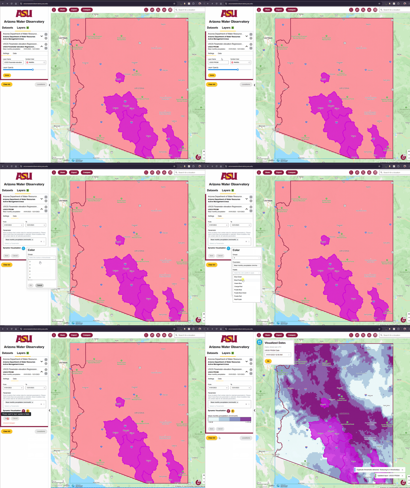
In the Layers tab, expand the PRISM layer and open “Settings.” Rename the layer to “USGS PRISM.” Open the “Data” tab and confirm the parameter is set to “mean monthly precipitation.” Under Dynamic Visualization, set “Groups” to 5 and choose “Blue-Purple.” Click “OK,” then “Save.” After a moment, the PRISM data will appear in the display. Note that the groups may self-adjust based on data values.
Exploring the data
The “Visualized Dates” panel in the upper left lets you step through monthly precipitation snapshots. Start with January 2023, then toggle to May and November, and watch how the patterns shift both in the data values and in where rain fell across the state.
Zoom into the Prescott AMA in central Arizona, as an example (you may then turn off the AMA in the legend to visualize PRISM easier). It received notably more average rainfall in May than it did in January, and far less in November. The distribution within the AMA also shifts month-to-month. If you switch to a satellite basemap and tilt into 3D view, we can learn why. Two mountain ranges flank the Prescott Valley, and in Arizona, higher elevations generally receive more precipitation. That topographic relationship, easy to miss on a flat map, becomes immediately visible in 3D. Click individual PRISM cells to see exact monthly values for specific locations.
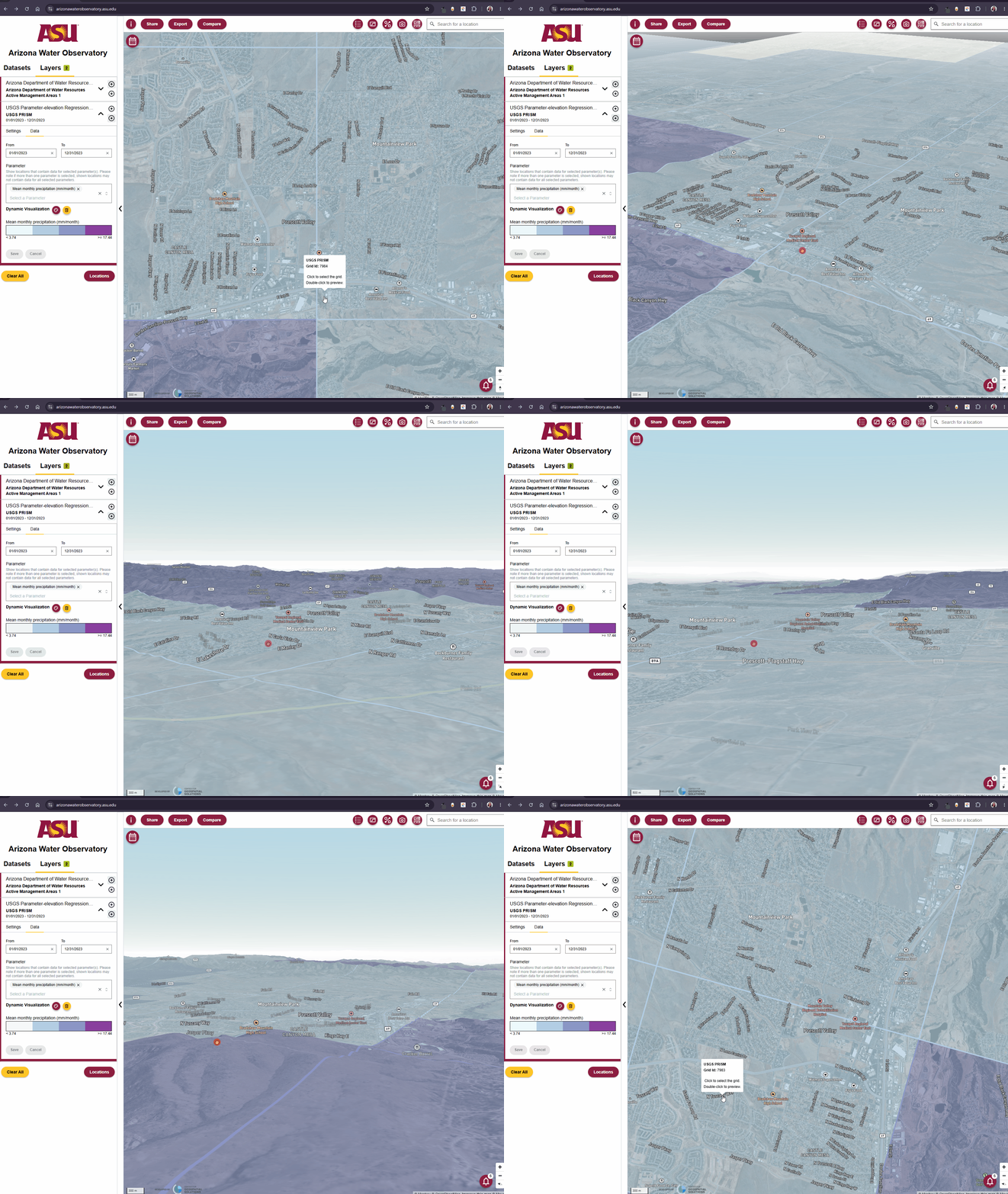
In the “Visualized Dates” dropdown you may switch between months to compare precipitation patterns; this displays November. To enter 3D view, right-click and slowly drag your mouse upward. To return to the standard view, click the compass in the lower right and drag your mouse downward.
What this makes possible
Layering regulatory boundaries over temporal precipitation data, exploring spatial patterns in 3D, clicking through to cell-level values — what we’ve done in a few minutes would typically require assembling data from multiple portals, reconciling formats, and doing the spatial work in a separate GIS environment. The AWO does this work for you.
This matters because smart water decisions rarely rely on a single dataset. Understanding how precipitation variability intersects with groundwater regulation or land use – an example of the complex reality Arizona’s water stewards navigate amid a backdrop of Colorado River negotiations, groundwater reforms, and long-term planning uncertainty — requires the kind of multi-variable, basin-scale view the AWO is designed to support.
This walk through is just the beginning. For a more intermediate, code-based approach using a groundwater example, see here. Or, for a surface water example using the AWO’s built in comparison feature, see here. Additional exercises and walkthroughs are available in the User Guide.